Neurons
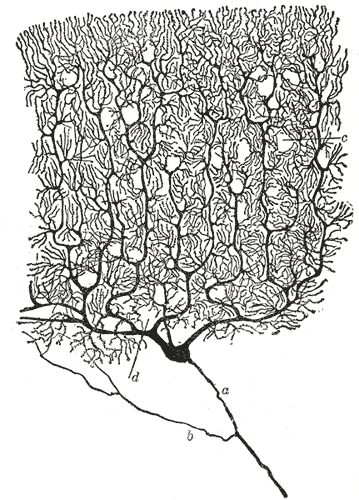
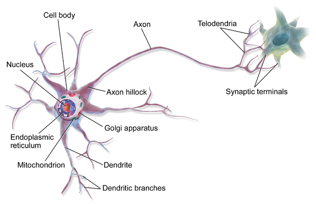
Our brains are composed of several types of cells, of which the most important for information processing is the Neuron. While there are several types of neurons with varying morphology, the canonical neuron has a tree-like branching structure called the dendritic tree, which is covered in synapses, a cell body (or soma) and a single axon. The dendrites and axon are extrusions of the cell wall membrane.
Modeling networks of biological neurons mathematically and computationally is a large and active research field. The current state-of-the-art models incorporate a great deal of biological detail - for example, modeling molecular interaction pathways of proteins, neurotransmitter and ion concentrations, growth and decay of synapses, dendrites and axons and electrochemical spike propagation. See this video for one example2.
However, back in the 1940s, some of the first simple neural network models simply ignored individual spikes and represented the mean firing rate of spikes as a single numeric rate. Neurons themselves were modeled as if they ‘fire’ if a threshold of activity from incoming spike rates is exceeded, which each incoming firing rate weighted by a scaling factor to represent the aggregate effect of the dendritic tree and the synapses.
Needless to say, this is a gross simplification of the biological reality. However, these simple neural network models were studied in their own right from a mathematical perspective and gave rise to what is now termed Artificial Neural Networks (ANNs) - with the understanding that, aside from the name, they have little to do with actual biological neural networks.
So, why are ANNs useful in machine learning?
Line fitting
Lets explore the simple mathematics behind a common artificial neuron. Recall from school, that there is a method for fitting a straight line to points on an x,y plot such that it is the ‘best fit’ in some sense. In trivial case where all the points actually lie on a line (co-linear), it is a simple matter of drawing a line through them:
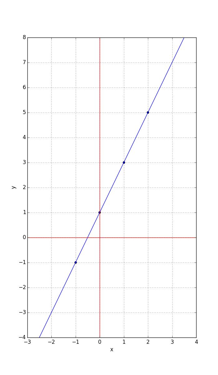
Here, the points are: (-1,-1), (0,1), (1,3) and (2,5)
Recall that the equation of the line can be represented in terms of the slope w (change in y over change in x) and intercept with the y-axis b (we could have used the more conventional a & b, but we’ll use w for slope, or weight and b for intercept, or bias, as weight and bias are the conventional ANN terms):
y = wx + b
In this example, using the upper right two points to compute the slope, we obtain:
w = (5 - 3) / (2 - 1) = 2
b = 1
Hence, the equation for the line is:
y = 2x + 1
Estimating parameters
The weight (w) and bias (b) above are known as the parameters of the line. Now, imagine that instead of the points plotted above, we actually obtained the points from a physical process of measurement from some type of sensor.
For example, suppose that y was the output of a robot sensor at different positions x and we knew from the physics of the situation that the relationship between x and y is linear (maybe y is proportional to a laser-beam time-of-flight for determining the distance to a target - since the speed of light is effectively constant, the one-way time-of-flight will be linearly proportional to the distance away).
Unfortunately, sensors aren’t perfect, so we might get slightly noisy y measurements from our sensor and hence the set of x,y pairs we obtain won’t be exactly co-linear. The question is, how can we estimate the best parameters (w & b) such that the line fits the data with the minimum amount of error (by some criteria we decide upon)?
One common technique, is known as Ordinary Least Squares fitting, or OLS. It minimizes the sum of squares of the errors. That is, it finds w and b such that if we sum all the differences (errors) between the ‘predicted’ y (lets call it yp = wx + b) and the actual measured y’s, it cannot be any smaller for any other values of w and b.
Suppose we measured the following x, y pairs from our sensor:
 x        y
-1    -1.208379
 0     0.971867
 1     1.931902
 2     5.820135
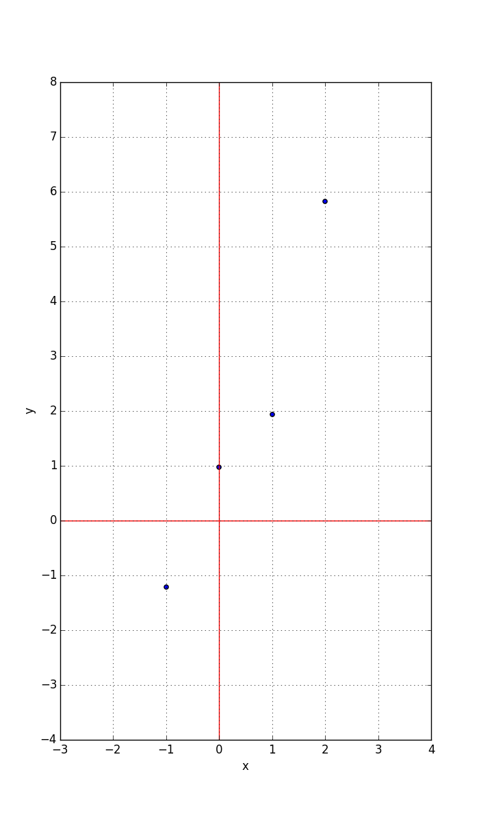
Clearly, the points are not exactly co-linear due to the noise in the y values.
We can plot an error surface that shows the sum of square differences between y and yp for many combinations of w and b:
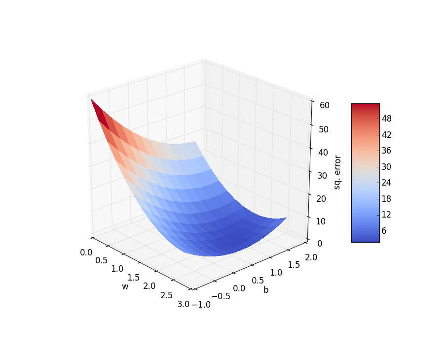
Keeping in mind that varying the w changes the slope of the line and varying b moves the line up and down, the ‘floor’ of this 3D plot represents all combinations of values for w and b over an area of w in [0 .. 3] and b in [-1 .. 2]. For each value of w and b the yp is computed by plugging the x values from the table above into the line equation wx + b and summing the squared differences from those values to the measured y values in the table above.
For example, to evaluate the squared error at w=1.5 and b=1:
 x        y        1.5x+1       (y - 1.5x+1)^2
-1    -1.208379    -0.5         0.501800807641
 0     0.971867     1           0.000791465689
 1     1.931902     2.5         0.322735337604
 2     5.820135     4           3.312891418225
                         Total = 4.138219029159 (Sum of Square errors)
Now, we want to find which w and b have the least error - which means the lowest point on the graph. This is a standard minimization problem for which many algorithms exist. One of the simplest classes are the Gradient Descent methods. Roughly, they start at some random point in the w,b space and compute the gradient (slope) of the surface and then take a step ‘down hill’. This is repeated until converging at the bottom - which in this example is at approx. w = 2.2046 and b = 0.7766 (which I determined using the Python SciPy StatsModels OLS functions).
If we plot the line y = 2.2046 x + 0.7766 over our measured x, y points, we obtain:
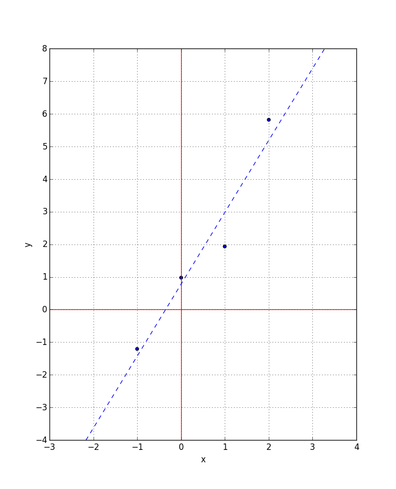
This is the line that best fits the measured data (with respect to the squared-error ‘cost’ measure).
A fancy name for curve fitting is regression (and mathematicians consider a line to be a special case of a curve - that just happens to have constant slope everywhere).
A single-neuron ANN
Artificial Neural Networks are typically represented graphically by drawing a circle for each neuron, with multiple inputs coming into one side (usually the left) and one output line leaving the other (usually the right side). Generally, a neuron sums its weighted inputs and applies an activation function to that sum to obtain the output.

Consider a very simple ‘network’ with only a single neuron. It will have two inputs x1 and x2, two weights w1 and w2 and use the identity function as an activation function (i.e. a function that has no effect). We’ll name the output y rather than o as above. Hence, the equation representing the single neuron will be:
y = w1 x1 + w2 x2
Now, if we fix w2=1 and x2 = b and let w1 be just w we have:
y = wx + b
Which is exactly the equation for a straight-line we saw above!
That is to say, a single-layer ANN is just performing a linear prediction of y from its inputs x for a given set of weights!
To ‘train’ a neural network such as this, we’re aiming to find a set of weights (parameters) such that the output is closest to the desired output for all given training input,output pairs (x,y pairs) with respect to a given cost measure. If we choose a squared-error measure and employ a Gradient Descent solver, we’ll arrive at a set of weights that represent a best fit exactly the same as our OLS regression example above.
If we were to add an extra input, then we’d be fitting a plane through a 3D space, instead of a line through a 2D space. More inputs generalize into higher dimensions (though our feeble brains, adapted to our 3D world, can’t visualize beyond 3 dimensions). For every input added, that implies an additional weight parameter and hence the error function surface is also a high-dimensional function in general. Typically deep networks have millions or billions of weight parameters and hence require a lot of training data to solve to reasonable weight values. In higher-dimensional spaces, the error function is far more complex with many ‘hills’, ‘peaks’ and ‘valleys’ making the task of finding an optimal global minimum far more challenging and typically in impractical. Gradient Descent based methods are are local optimization techniques - they may get ‘stuck’ in a local minimum rather than finding the global minimum. However, it has been discovered empirically, that for real-world problems the global optimal is often reached or that local optima are often still ‘good enough’ solutions to the problem at hand. There is an entire subfield of mathematics devoted to optimization.
Logistic regression
Logistic regression is a fancy name given to line fitting where an additional function - the, so called logistic function - is applied to the linear output. For example:
y = s(wx + b)
where s(.) is the logistic function, which looks like a squashed S-shape, or sigmoid, and is defined by:
s(t) = 1 / (1 + e^-t)
(where ‘^’ is the power operator and hence, e^-t is alternative notation for e-t; and e is Euler’s number - the base of the natural logarithms and approximately e=2.71828)
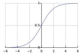
Logistic regression has a long history in statistics and is often used when the predictor (y) should be a probability, which must be between [0 .. 1]. As you can see, it maps whatever value wx + b evaluates to, into the range [0 .. 1] and hence is suitable as a probability value. ANNs often utilize the logistic/sigmoid function as the activation function for this reason and it provides a means for creating networks that perform classification - where any given output is a probability that the input belongs to a given category, or class.
Multi-layer ANNs
A Neural network with only one ‘layer’ of neurons, as depicted above, can represent a linear relationship between its inputs and outputs (if it uses a ‘linear’ / identity activation function). However, the types of relationships found in typical problems to which ANNs are applied are highly non-linear. One way to dramatically extend the set of functions that an ANN can represent, is to use multiple layers. In fact, it has been shown mathematically, that ANNs can represent any possible functional mapping from inputs to outputs (limits on numerical accuracy/resolution not withstanding) - they are universal function approximators3,4.
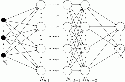
ANNs can have arbitrary many layers.
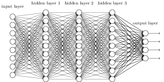
5-layer ANN.
We’ll return to Neural Networks once we’ve reached the stage of being able to implement the necessary forward multiplication and addition computations using hardware logic circuits.
-
Neuron, Wikipedia, Accessed 2015-06-26. ↩ ↩2
-
Whole Brain Catalog, Mark Ellisman, Center for Research in Biological Systems (CRBS), The University of California, San Diego. Animated by Drew Berry, molecularmovies.com. Accessed 2015-06-21. ↩
-
Universal Approximation Theorem, Wikipedia. Accessed 2015-06-27. ↩
-
Balázs Csanád Csáji. Approximation with Artificial Neural Networks; Faculty of Sciences; Eötvös Loránd University, Hungary ↩